

Correlation seems simple on the surface. As one thing gets larger, something either gets larger or smaller. While at a high level, this is generally true, once we go further into correlation, there is much more it can tell us.
This 5-minute read will cover what correlation is, why a correlation analysis is important in data mining, how to detect and handle Multicollinearity, and some neat tricks that may improve your models.
You won’t want to miss this one.

What is correlation in data analysis?
Correlation is simply how one thing affects another. If A increases when B increases, they are said to have a positive correlation. If A decreases when B increases, they are said to have a negative correlation.
As data scientists, we generally do not care if the correlation coefficients between a feature and our target variable are positive or negative; we only care that our features affect our dependent variable.
One thing that you need to be careful about is the assumption that correlation equals causation.
Correlation vs. Causation
Just because one of your feature variables and your target variables are correlated does not mean that this feature is necessary or should be included in the final model/analysis.
For example, let’s say you were trying to figure out what variables were essential to how much people spend in your company’s store.
You plot them against each other, and the higher the fruit enjoyment is for that person, the more money they spend in the store.
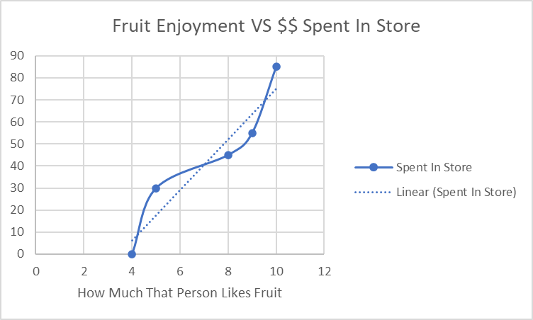
Based on this, you’d assume that fruit enjoyment is important to your analysis and keep it in your final model.
However, upon further investigation (with something like a chi-square test), you realize these two were correlated by chance, and the more someone enjoys fruit doesn’t change how much they’re going to spend in your store.
You’ve now seen Correlation vs. Causation in real-time – just because two things are correlated does not mean they have a causal relationship.
Positive Correlation
Now that you understand where to use correlation, we show what a positive correlation will look like below:
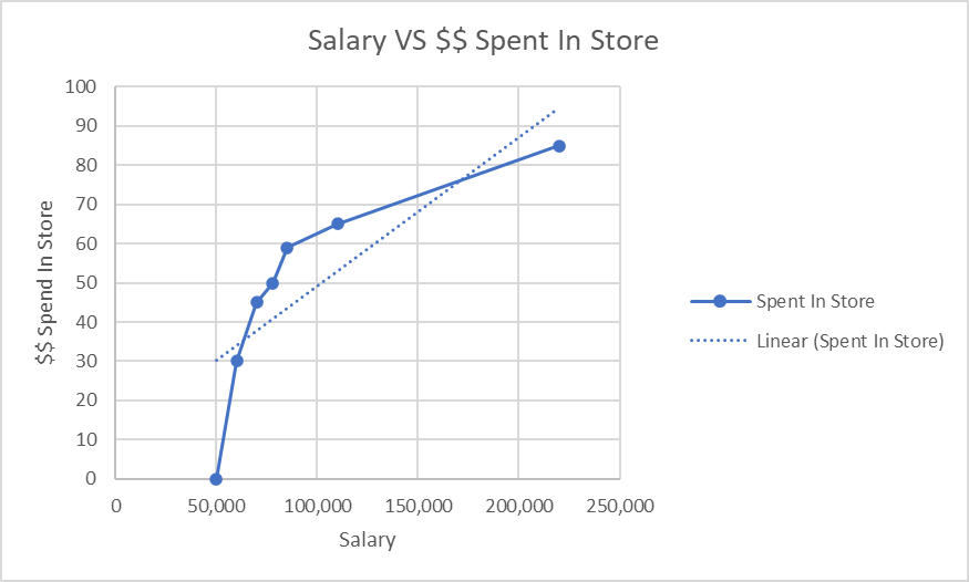
We can see that as salary increases, the amount that will be spent in our store also increases
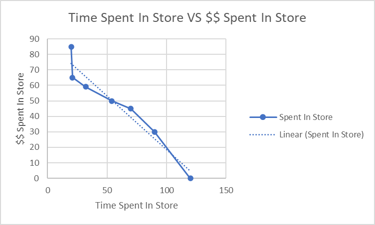
Negative Correlation
Contrast that with something below, where the longer someone spends in the store, the less they spend.
Why Correlation Analysis is Important In Data Science
While we’ve discussed the correlation between our feature and target variables, what happens when our features are correlated with each other in our raw data?
For example:
Correlation Analysis in Python
# check correlation
import pandas as pd
import seaborn as sns

# as always
# public data
# https://www.kaggle.com/datasets/uciml/red-wine-quality-cortez-et-al-2009
df = pd.read_csv('winequality-red.csv')

sns.heatmap(df.corr())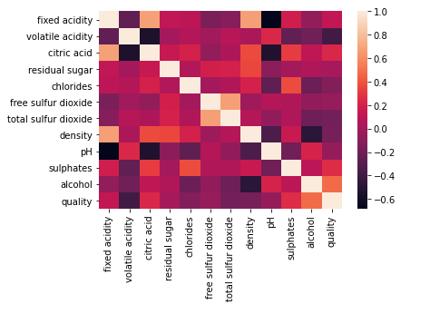
Right away, things like fixed acidity and density seem to be heavily correlated, which can cause serious problems down the road.
Understanding what correlational means in your data
Dealing with correlated features in your dataset is a whole branch of data mining. This idea of correlated “independent” features is called Multicollinearity and can usually be handled cleanly and quickly.
How to handle Multicollinearity in data mining?
Now that we know what Multicollinearity is, you can probably guess how we will handle it.
But first, we have to find it.
How to find Multicollinearity in your dataset with Python
Finding Multicollinearity in your dataset is tricky, but we have some tricks up our sleeves.
Personally, my favorite is the Variance Inflation Factor (VIF).
While the math is pretty dense, all you need to know is that the higher the VIF number, the more correlated that variable is with other features in our dataset.
While a VIF of one is generally what we want to see, you rarely get it. As a general guide, values less than three shouldn’t cause any concern. And Values higher than five are an immediate cause of concern and need to be dealt with.
Let’s head back to our dataset from above:
# check correlation
# public ds
import pandas as pd
from statsmodels.stats.outliers_influence import variance_inflation_factor

# as always
# public data
# https://www.kaggle.com/datasets/uciml/red-wine-quality-cortez-et-al-2009
df = pd.read_csv('winequality-red.csv')

# find multicollinearity in our dataset
# this function will work for any dataset
# make sure to save it
def find_vifs(dataset):

    # need a base dataset
    base_vif = pd.DataFrame()

    # this will be our rows
    base_vif['Columns'] = dataset.columns

    # calculate each of those values
    base_vif['VIF'] = [variance_inflation_factor(dataset.values, i) for i \
                      in range(dataset.shape[1])]

    # return it
    return base_vif

# lets send everything but our target variable to our function
print(find_vifs(df[[col for col in df.columns if col != 'quality']]))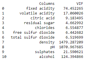
We see that only one of our variables passes our VIF test (residual sugar), and all of our others are much higher than five.
What do we do?
Well..
How to handle Multicollinearity for your models
Handling multicollinearity in a dataset is not an easy task but something you will have to do repeatedly as a data scientist.
My three favorite ways of handling multicollinearity are
- Dropping A Column (Least Favorite)
- Creating A New Column From Two Correlated Features
- Lasso Regression analysis
- Understanding the dataset
Dropping a column will work in situations where you have problematic data.
If you have a duplicate column, or some of the values from another column have overridden another, it’s probably best to eliminate one of those columns.
Creating a new column from two correlated features is a little more tricky.
While you want to ensure you’re handling the Multicollinearity, you want to ensure you’re not losing any variance in the data.
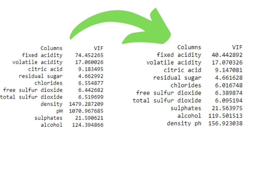
I improve our VIF readings (across the board) in this code by creating an interaction term between density and pH.
# check correlation
# public ds
import pandas as pd
from statsmodels.stats.outliers_influence import variance_inflation_factor

# copy of above dataframe
df_fix2 = df.copy()

# lets create a new interaction term
df_fix2['density_ph'] = df_fix2.density * df_fix2.pH

# drop the old terms
df_fix2.drop(['density','pH'], inplace=True, axis=1)

# find multicollinearity in our dataset
# this function will work over and over again (for smallerish sets)
# make sure to save it
def find_vifs(dataset):

    # need a base dataset
    base_vif = pd.DataFrame()

    # this will be our rows
    base_vif['Columns'] = dataset.columns

    # calculate each of those values
    base_vif['VIF'] = [variance_inflation_factor(dataset.values, i) for i \
                      in range(dataset.shape[1])]

    # return it
    return base_vif

# re-run our VIF
print(find_vifs(df_fix2[[col for col in df_fix2.columns \
                         if col != 'quality']]))
We see our improvements:
Another example of this could be a dataset with the amount of rainfall that falls every hour daily.
On rainy days, there will probably be a lot of rain every hour, and on non-rainy days there probably wouldn’t be much rain.
This dataset would show high Multicollinearity – but what if we combined all of those features into a variable: amount_of_rain_per_day?
This would preserve all of our data and quickly eliminate all of the multicollinearity problems from our dataset.
Finally, we can programmatically handle Multicollinearity.
While I’m not going to dive deep into what Lasso Regression is, know that it uses a regularization parameter to drive features to zero. We can use this for feature selection:
import pandas as pd
from sklearn.linear_model import Lasso
from sklearn.model_selection import GridSearchCV

# as always
# public data
# https://www.kaggle.com/datasets/uciml/red-wine-quality-cortez-et-al-2009
df = pd.read_csv('winequality-red.csv')

# run a lasso model
lasso = Lasso()

# split our dataset
X = df[[col for col in df.columns if col != 'quality']]
y = df['quality']

# define some params to search
params = {'alpha': [1e-15, 1e-10, 1e-8,
                    1e-4, 1e-3, 1e-2, 1, 1e1,
                    1e2, 1e3, 1e4, 1e5, 1e6, 1e7]}

# run through all of our params above
lasso_model = GridSearchCV(lasso, params,
                          scoring='neg_mean_squared_error',
                          cv=5)

# fit our model onto our dataset
lasso_model.fit(X, y)

# find our best estimator
lasso_best_params = lasso_model.best_estimator_

# lets refit just that model, so we can see our features
lasso_best_params.fit(X, y)

# our params below
print(lasso_best_params.coef_)
Our Lasso struggled a bit, only able to drive one feature entirely to zero.

Let’s see if we can continue to make improvements on our VIF scores
We filter out any coefficient that does not have a higher value absolute value than .01.
# lets take anything with an abs value > .01
mask = [True if abs(val) > .01 else False for val in lasso_best_params.coef_]

# filter down to our correct columns
df_filtered = X.iloc[:,mask]

# preview of our dataframe below
df_filtered.head()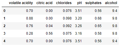
Now that we have our dataset, we can use our VIF function to check and see if our Multicollinearity has improved.
## finally, lets check our VIF
def find_vifs(dataset):

    # need a base dataset
    base_vif = pd.DataFrame()

    # this will be our rows
    base_vif['Columns'] = dataset.columns

    # calculate each of those values
    base_vif['VIF'] = [variance_inflation_factor(dataset.values, i) for i \
                      in range(dataset.shape[1])]

    # return it
    return base_vif

# lets send everything but our target variable to our function
print(find_vifs(df_filtered[[col for col in df_filtered.columns \
                             if col != 'quality']]))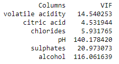
We still cannot get all of our VIFs into the range we wanted.
This brings me to my final and last way of handling Multicollinearity: understanding the data.
If you’ve noticed the column’s name throughout this project, you’ll see that this dataset is a listing of all the chemicals within some “drink.”
When one chemical goes up, another goes down, which causes a reaction in another, etc. (I’m no chemist)
In some situations, no matter what you do – your dataset will have Multicollinearity.
Sometimes that is okay; make sure you choose methods and models that can handle this sort of thing (Tree methods and a few others).
Final Thoughts on a correlation analysis in data mining
Throughout this post, we’ve learned what correlation is, how it can help you in your data mining projects, what too much correlation can bring to your datasets, and how to handle it.
Correlation is a fundamental piece of statistical analysis and data science. Hopefully, you now have another tool in your ever-expanding data mining toolbox!