

As data scientists, we’re interested in solving future problems. We do this by finding patterns and trends in data, then applying these insights in real-time. Bayes theorem (the backbone of Bayes Classification) is built upon class-level prior probability, and this is perfect since the prior probability is created from previous events (our data).
This 4-minute read will cover how to code a couple of classifiers using the Bayes theorem in python, when it’s best to use each one, and some advantages and disadvantages.
This is a pivotal family of algorithms, don’t miss out on this one.

What is Bayes classification in data mining?
When someone says Bayes classification in data mining, they are most likely talking about the Multinomial Naive Bayes Classifier. This classification algorithm works great on text data and training sets with low amounts of training data. There are other types of Naive Bayes classifiers, like the Bernoulli and Gaussian.
When Thomas Bayes passed away in 1761, many of the minister’s documents were released.
Hidden in some of these documents was the discovery of Bayes’ Theorem.
Due to the low computational power back then (no computers) and math and statistics being done by hand, Bayes’ Theorem wasn’t seen as a breakthrough at the time.
However, Later in the 20th century, when we saw substantial computational advances, we finally realized how powerful this discovery was.
What is the Bayes Theorem?
Bayes’ theorem, at its core, is the idea that we can utilize prior probabilities to give future insights into things that haven’t happened yet. Bayes classification is built upon the ideas in the Bayes theorem.
We must first understand conditional probability to understand the brilliance behind Bayes’ theorem.
Let’s rebuild the Bayes Theorem from scratch.
Below, we have a picture of the conditional probability formula for A given B:
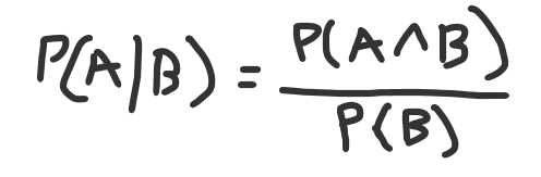
A given B equals the intersection of A and B, divided by the probability of B.
Let’s continue down this path, and since we have the prior probabilities and the intersections, we can calculate B given A:
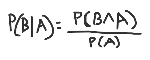
B given A equals the intersection of A and B, divided by the probability of A.
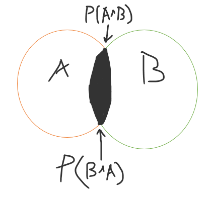
These are just formulas. The problem with these formulas is it’s generally pretty difficult to calculate P (A ∩ B) or P (B ∩ A ), and we need a way around that.
When it comes to the intersection (think of it as an inner join in SQL), it does not matter which order you write it in; mathematically, it will be the same.
P (A ∩ B) = P (B ∩ A ) !!
Building on that idea above, we can finally finish deriving the Bayes Theorem.
Since we know our conditional probability formulas, we write those first.
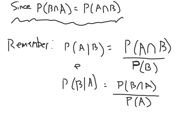
We can multiply the denominator over for both of these, and we arrive at:
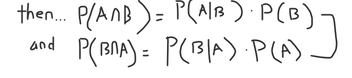
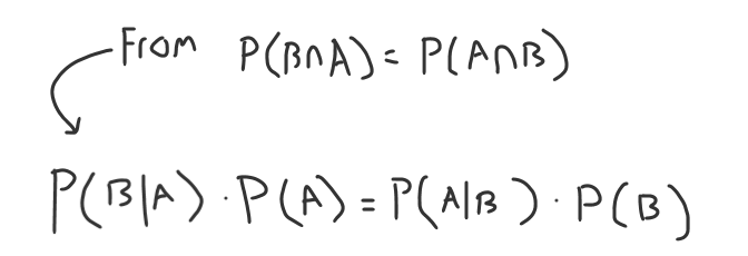
Now, if we remember from above, the intersections are equal.
P (A ∩ B) = P (B ∩ A ) -> P(A|B) * P(B) = P(B|A) * P(A)
We replace each side of the intersection formula with the formulas above.
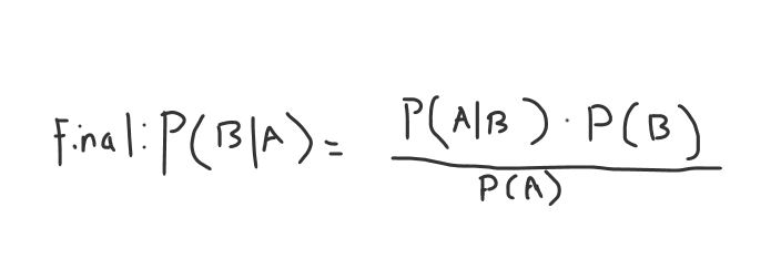
We could pick either side of the equation to finalize since you have B given A or A given B.
Now, we can make the final move towards Bayes Theorem and divide over our probability of A to get B given A.
(You could also do A given B)
Why is the Bayes Theorem better than conditional probability in data mining?
The main benefit of the Bayes theorem compared to conditional probability is that the Bayes theorem does not use the intersection of the two sets. While the Bayes Theorem is derived from conditional probability, this subtle difference means our dataset has all we need to build our classifier.
The Types of Naive Bayesian Classifiers Used in Data Mining
The different types of Naive Bayesian Classifiers are:
- Multinomial
- Gaussian
- Complement
- Bernoulli
- Flexible Bayes
- Categorical
- Out-Of-Core
When should you use Multinomial Naive Bayes?
Multinomial Naive Bayes is the most commonly used Bayes Classifier. This classifier is predominantly used in text analysis (like spam detection) but can be used in any multivariate binomial situation. To utilize Multinomial Naive Bayes, you’ll need clean labeled data to calculate the prior probabilities.
(Four coded Naive Bayes Classifiers Below)
How To Code Multinomial Naive Bayes in Python
# email spam
# as always, public dataset
# https://www.kaggle.com/datasets/uciml/sms-spam-collection-dataset
import pandas as pd
import numpy as np

# load in our dataset
df = pd.read_csv('spam.csv', encoding='latin-1')

# lets rename the columns, and drop
df.columns = ['Target','Text','1','2','3']
df = df.drop(columns=['1','2','3'])

# replace our target with model ready values
df['Target'] = df['Target'].replace({'ham':0,'spam':1})

df.head()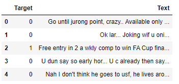
This text data is a little messy, we get rid of stop words, numbers, and emails.
# lets quickly clean and tokenize text
# for modeling
import string
import nltk

def cleaning_function(text):

    # remove numbers, replace with blank
    text = text.replace(r'/d+','')

    # lets remove emails since
    # its an email classifier
    # replace with blank
    text = text.replace(r'S*@\S*\s?','')

    #lower the words
    text = text.lower()

    # tokenize each word
    arr = nltk.word_tokenize(text)

    # we dont want punctuation or stop words
    bad_words = nltk.corpus.stopwords.words('english')+list(string.punctuation)

    # lets now final clean each array
    word_vec = []

    # here i use w instead of word so it fits on screen
    # usually I like to use word instead of w
    for w in arr:
        if w and w.isalpha() and w not in bad_words:
            word_vec.append(w)


    # return the array as a string, and remove extra spacing on end
    return ' '.join(word_vec).strip()


# apply our cleaning function
df['Text'] = df['Text'].apply(cleaning_function)

# lets see what it looks like
df.head()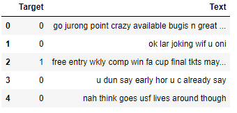
Let’s create our word embeddings using the term frequency-inverse document frequency.
from sklearn.feature_extraction.text import TfidfVectorizer
from sklearn.model_selection import train_test_split

# term frequency inverse
tf_idf = TfidfVectorizer(max_features=2500)

# for a production system, you'd want to split
# before applying tf_idf, to prevent data leakage
# to keep things short, i'm going to continue on
X = tf_idf.fit_transform(df['Text']).toarray()

# split out our y
y = df['Target'].values

# random_state 32 incase you're following along
# 10% data held out for testing
X_train,X_test,y_train,y_test = train_test_split(X,y,test_size=0.1,\
                                                 random_state=32)
We can now run our model:
from sklearn.metrics import precision_score, recall_score, confusion_matrix, classification_report, f1_score
from sklearn.naive_bayes import MultinomialNB
# MultinomialNB
clf = MultinomialNB()
# fit our classifier
clf.fit(X_train, y_train)
# make predictions
pred = clf.predict(X_test)
# lets see a confusion_matrix
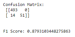
print(f'Confusion Matrix:\n {confusion_matrix(y_test, pred)}\n\n')
# and our F1 Score
print(f'F1 Score: {f1_score(y_test, pred)}')
We see our results below:
When to use Complement Naive Bayes Over Multinomial Naive Bayes
Complement Naive Bayes has shown to be a better classifier than regular Multinomial Naive Bayes whenever your target classes aren’t equally distributed. Complement Naive Bayes also sometimes outperforms Multinomial Naive Bayes on text classification tasks because of the way it handles feature independence.
Read more about it here in the original research paper.
How To Code Complement Naive Bayes in Python
# email spam
# as always, public dataset
# https://www.kaggle.com/datasets/uciml/sms-spam-collection-dataset
import pandas as pd
import numpy as np

# load in our dataset
df = pd.read_csv('spam.csv', encoding='latin-1')

# lets rename the columns, and drop
df.columns = ['Target','Text','1','2','3']
df = df.drop(columns=['1','2','3'])

# replace our target with model ready values
df['Target'] = df['Target'].replace({'ham':0,'spam':1})

df.head()
This text data is a little messy, we get rid of stop words, numbers, and emails.
# lets quickly clean and tokenize text
# for modeling
import string
import nltk

def cleaning_function(text):

    # remove numbers, replace with blank
    text = text.replace(r'/d+','')

    # lets remove emails since
    # its an email classifier
    # replace with blank
    text = text.replace(r'S*@\S*\s?','')

    #lower the words
    text = text.lower()

    # tokenize each word
    arr = nltk.word_tokenize(text)

    # we dont want punctuation or stop words
    bad_words = nltk.corpus.stopwords.words('english')+list(string.punctuation)

    # lets now final clean each array
    word_vec = []

    # here i use w instead of word so it fits on screen
    # usually I like to use word instead of w
    for w in arr:
        if w and w.isalpha() and w not in bad_words:
            word_vec.append(w)


    # return the array as a string, and remove extra spacing on end
    return ' '.join(word_vec).strip()


# apply our cleaning function
df['Text'] = df['Text'].apply(cleaning_function)

# lets see what it looks like
df.head()
Let’s create our word embeddings using the term frequency-inverse document frequency.
from sklearn.feature_extraction.text import TfidfVectorizer
from sklearn.model_selection import train_test_split

# term frequency inverse
tf_idf = TfidfVectorizer(max_features=2500)

# for a production system, you'd want to split
# before applying tf_idf, to prevent data leakage
# to keep things short, i'm going to continue on
X = tf_idf.fit_transform(df['Text']).toarray()

# split out our y
y = df['Target'].values

# random_state 32 incase you're following along
# 10% data held out for testing
X_train,X_test,y_train,y_test = train_test_split(X,y,test_size=0.1,\
                                                 random_state=32)
We can now run our model:
from sklearn.metrics import precision_score, recall_score, confusion_matrix, classification_report, f1_score
from sklearn.naive_bayes import ComplementNB

# ComplementNB
clf = ComplementNB()

# fit our classifier
clf.fit(X_train, y_train)

# make predictions
pred = clf.predict(X_test)

# lets see a confusion_matrix
print(f'Confusion Matrix:\n {confusion_matrix(y_test, pred)}\n\n')

# and our F1 Score
print(f'F1 Score: {f1_score(y_test, pred)}')
Interesting results below:
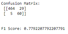
While our F1 Score overall is lower than Multinomial, our false positive rate is much lower.
You may prefer this model in some situations where a false positive is much worse than a false negative.
When should you use Gaussian Naive Bayes?
The Gaussian Naive Bayes classifier should be used when your continuous features are normally distributed. Even if your features aren’t exactly normal, Gaussian Naive Bayes will still give better results than Multinomial Naive Bayes.
Gaussian Naive Bayes plays a massive role in data science, as continuous features can usually be transformed into normality.
If you’re confused about normality, our articles on the chi-square test and QQ Plot should help.
How To Code Gaussian Naive Bayes In Python
# email spam
# as always, public dataset
# https://www.kaggle.com/datasets/uciml/sms-spam-collection-dataset
import pandas as pd
import numpy as np

# load in our dataset
df = pd.read_csv('spam.csv', encoding='latin-1')

# lets rename the columns, and drop
df.columns = ['Target','Text','1','2','3']
df = df.drop(columns=['1','2','3'])

# replace our target with model ready values
df['Target'] = df['Target'].replace({'ham':0,'spam':1})

df.head()
This text data is a little messy, we get rid of stop words, numbers, and emails.
# lets quickly clean and tokenize text
# for modeling
import string
import nltk

def cleaning_function(text):

    # remove numbers, replace with blank
    text = text.replace(r'/d+','')

    # lets remove emails since
    # its an email classifier
    # replace with blank
    text = text.replace(r'S*@\S*\s?','')

    #lower the words
    text = text.lower()

    # tokenize each word
    arr = nltk.word_tokenize(text)

    # we dont want punctuation or stop words
    bad_words = nltk.corpus.stopwords.words('english')+list(string.punctuation)

    # lets now final clean each array
    word_vec = []

    # here i use w instead of word so it fits on screen
    # usually I like to use word instead of w
    for w in arr:
        if w and w.isalpha() and w not in bad_words:
            word_vec.append(w)


    # return the array as a string, and remove extra spacing on end
    return ' '.join(word_vec).strip()


# apply our cleaning function
df['Text'] = df['Text'].apply(cleaning_function)

# lets see what it looks like
df.head()
Let’s create our word embeddings using the term frequency-inverse document frequency
from sklearn.feature_extraction.text import TfidfVectorizer
from sklearn.model_selection import train_test_split

# term frequency inverse
tf_idf = TfidfVectorizer(max_features=2500)

# for a production system, you'd want to split
# before applying tf_idf, to prevent data leakage
# to keep things short, i'm going to continue on
X = tf_idf.fit_transform(df['Text']).toarray()

# split out our y
y = df['Target'].values

# random_state 32 incase you're following along
# 10% data held out for testing
X_train,X_test,y_train,y_test = train_test_split(X,y,test_size=0.1,\
                                                 random_state=32)
We can now run our model:
from sklearn.metrics import precision_score, recall_score, confusion_matrix, classification_report, f1_score
from sklearn.naive_bayes import GaussianNB

# GaussianNB
clf = GaussianNB()

# fit our classifier
clf.fit(X_train, y_train)

# make predictions
pred = clf.predict(X_test)

# lets see a confusion_matrix
print(f'Confusion Matrix:\n {confusion_matrix(y_test, pred)}\n\n')

# and our F1 Score
print(f'F1 Score: {f1_score(y_test, pred)}')
Interesting results below:

This model struggled, but do we know why?
Remember, Gaussian Naive Bayes assumes our features have an underlying normal distribution.
Our TFIDF Vectors are not normal. These results are to be expected.
When should you use Bernoulli Naive Bayes?
You should use the Bernoulli whenever your features have an underlying Bernoulli distribution. One of the easiest ways to identify this is if your features are binary, with only two options, zero and one. However, this model does very well with vectorized text data.
Remember, these columns have to be independent of one another and shouldn’t be utilized on a binary dataset from things like one hot encoding and creating dummy variables.
How To Code Bernoulli Naive Bayes In Python
# email spam
# as always, public dataset
# https://www.kaggle.com/datasets/uciml/sms-spam-collection-dataset
import pandas as pd
import numpy as np

# load in our dataset
df = pd.read_csv('spam.csv', encoding='latin-1')

# lets rename the columns, and drop
df.columns = ['Target','Text','1','2','3']
df = df.drop(columns=['1','2','3'])

# replace our target with model ready values
df['Target'] = df['Target'].replace({'ham':0,'spam':1})

df.head()
This text data is a little messy, we get rid of stop words, numbers, and emails.
# lets quickly clean and tokenize text
# for modeling
import string
import nltk

def cleaning_function(text):

    # remove numbers, replace with blank
    text = text.replace(r'/d+','')

    # lets remove emails since
    # its an email classifier
    # replace with blank
    text = text.replace(r'S*@\S*\s?','')

    #lower the words
    text = text.lower()

    # tokenize each word
    arr = nltk.word_tokenize(text)

    # we dont want punctuation or stop words
    bad_words = nltk.corpus.stopwords.words('english')+list(string.punctuation)

    # lets now final clean each array
    word_vec = []

    # here i use w instead of word so it fits on screen
    # usually I like to use word instead of w
    for w in arr:
        if w and w.isalpha() and w not in bad_words:
            word_vec.append(w)


    # return the array as a string, and remove extra spacing on end
    return ' '.join(word_vec).strip()


# apply our cleaning function
df['Text'] = df['Text'].apply(cleaning_function)

# lets see what it looks like
df.head()
Let’s create our word embeddings using the term frequency-inverse document frequency.
We reference data leakage in this snippet of code; more can be found in that link.
from sklearn.feature_extraction.text import TfidfVectorizer
from sklearn.model_selection import train_test_split

# term frequency inverse
tf_idf = TfidfVectorizer(max_features=2500)

# for a production system, you'd want to split
# before applying tf_idf, to prevent data leakage
# to keep things short, i'm going to continue on
X = tf_idf.fit_transform(df['Text']).toarray()

# split out our y
y = df['Target'].values

# random_state 32 incase you're following along
# 10% data held out for testing
X_train,X_test,y_train,y_test = train_test_split(X,y,test_size=0.1,\
                                                 random_state=32)
We can now run our model:
from sklearn.metrics import precision_score, recall_score, confusion_matrix, classification_report, f1_score
from sklearn.naive_bayes import BernoulliNB

# BernoulliNB
clf = BernoulliNB()

# fit our classifier
clf.fit(X_train, y_train)

# make predictions
pred = clf.predict(X_test)

# lets see a confusion_matrix
print(f'Confusion Matrix:\n {confusion_matrix(y_test, pred)}\n\n')

# and our F1 Score
print(f'F1 Score: {f1_score(y_test, pred)}')
Interesting results below:
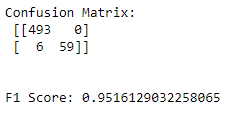
Bernoulli Naive Bayes Classifier was by far our best classifier, with very low False positives and no false negatives.
Other Relevant Data Science Python Tutorials
We have a ton of additional Data science python tutorials built just like this one.
This will help you better understand machine learning and the different ways you can implement these algorithms in python.
Links to those articles are below:
- Stratified Sampling in Python: While we just used train test split, in this article, stratified sampling could have been used.
- Full Multivariate Polynomial Regression Python Code: Like this breakdown, we go over Polynomial Regression with a fully coded python solution.
When should you use Bayesian Classification Over Other statistical classifiers?
The biggest advantage of using Naive Bayes is that it does not need much training data. Prior Probabilities converge quickly to their actual values, and approximate values obtained from small datasets will still do well in classification.
Also, due to its fast computation and many variations, Naive Bayes is a great starting point for any classification problem.
I like using Naive Bayes as a base algorithm to explore my dataset, but I will usually move on to something more powerful, like a gradient-boosted classifier, if it makes sense.

Always check your ROC curve with cross-validation to determine which classifier works best for you!
If you need more than this, Here is a fascinating paper from 2006 comparing multiple variations of Naive Bayes for spam classification.
After the study had concluded, The researchers were most impressed by the performance of multinomial Bayes with Boolean values.
This could be something to try if you’re struggling with either performance or computation.