

When it comes to classification problems, your population data is critical. While investigating our target class, we often notice disproportionate sampling. In these instances, what do we do?
The Stratified sampling technique means that your sample data will have the same target distribution as your population data. In this instance, your primary dataset will be seen as your population, and the samples drawn from it will be used for training and testing.

Complete coding walk-through at the bottom of the page
What is stratified sampling in Machine Learning?
Understanding stratified sampling is simple. When sampling to create your models and datasets, you want your training set and test datasets to resemble your population data accurately.
Since we operate under the assumption that our population data is as close as we will get to real-world data, simple random sampling could create unbalanced classes that do not accurately resemble our population.
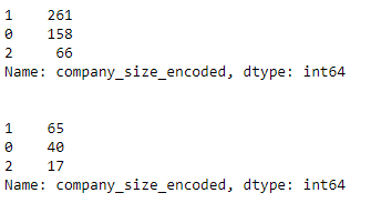
For example, look at this training set and test datasets derived from the same population.
We then apply a stratified sampling technique.
While the numbers are much higher by count in our initial training set (the first set of values), both sets of values follow the original population distribution.
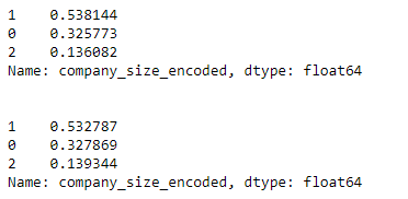
If we look at these as a percentage, instead of a total count of each – we again notice they are the same distribution.
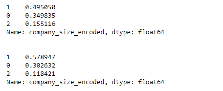
Here we see this compared to randomly sampled data, where the training and test datasets seem to be from different distributions (they aren’t).
From experience, stratified sampling works best when there is more than one class, and the classes aren’t very unbalanced.
When you run into scenarios where one class dominates the other, you will probably need a different sampling method.

When should you not use stratified sampling?
You should not use stratified sampling when you have a very small dataset.
Stratified sampling aims to mimic the distributions within our population to create accurate models.
However, if the number of rows in our dataset is not sufficient, we can not make the underlying assumption that our population accurately represents the real world.
In these scenarios, a random sampling technique would prove superior, or a sampling method that has replacement.
It’s best to utilize cross-validation and find what works best for you and your data.
![]()
How is stratified sampling calculated?
Stratified sample data is calculated from the target class distribution in percentages. For example, if you have a population with 80% Y and 20% N for your target class, your sample distribution will also be 80% Y and 20% N, no matter how large that sample is.
What is the difference between Random sampling and Stratified Sampling?
The difference between Random Sampling and stratified sampling is that random sampling grabs random samples from the dataset, while stratified sampling chooses based on criteria. Random sampling doesn’t care about the final distribution of the sample data, whereas stratified sampling will mimic the population distribution as close as possible.
Both of these sampling techniques are under the assumption that your data is independent, where you can grab from the population freely.
How to perform stratified sampling to improve the performance of machine learning algorithms
While I believe there is validity in multi-class situations with lots of data, you will not have this luxury in most real-world scenarios.
I’ve seen model improvements using randomly sampled data, and I’ve also seen improvements using stratified sampling techniques.
What’s important is that we create homogeneous subgroups between classes.
Let’s see how we would do it.
Performing Stratified Sampling in Sklearn
from sklearn.model_selection import train_test_split

# train test split logic
# note that stratify=y
X_train, X_test, y_train, y_test = train_test_split(X, y,
                                                   test_size=0.5,
                                                   stratify=y)

# we see our training set follows the same distribution
print(y_train.value_counts(normalize=True), '\n\n')

# we see our test set follows the same distribution
print(y_test.value_counts(normalize=True))
Notice how close the training and test distributions are in our test and train set.
Performing Random Sampling (Getting Random Samples) in Sklearn
# train test split logic
from sklearn.model_selection import train_test_split

# note that stratify is left out in this one
X_train, X_test, y_train, y_test = train_test_split(X, y,
                                                    test_size=0.5)

print(y_train.value_counts(normalize=True), '\n\n')

print(y_test.value_counts(normalize=True))
Notice how training and test distributions seem like they’re from different populations.
Performing Stratified sampling in Pandas
# performing Stratified Sampling With Pandas and Numpy
import pandas as pd
import numpy as np
# lets say we wanted to shrink our data frame down to 125 rows,
# with the same
# target class distribution
size = 125
# using groupby and some fancy logic
stratified = df.groupby('company_size_encoded', group_keys=False)\
.apply(lambda x: \
x.sample(int(np.rint(size*len(x)/len(df)))))\
.sample(frac=1).reset_index(drop=True)
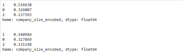
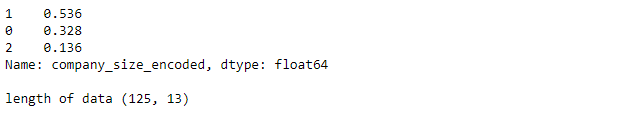
# we can see that our sample is 125 rows,
# while our distribution follows as close as possible
print(stratified.company_size_encoded.value_counts(normalize=True),\
f'\n\nlength of data {stratified.shape}')
While we have shown that this is possible in pandas, I highly recommend you stick to Sklearn for sampling.
Does stratified sampling improve models?
Let’s try creating a test to figure this out.
We will take the same dataset and problem and apply the same transformations.
The only difference will be if we use stratified or random sampling when building our training and test sets.
We will compare the test accuracy using Matthews Correlation Coefficient and see if our stratified sampling made a difference.
This is a complete data science/machine learning pipeline. While feature engineering is a little weak, most projects flow in this nature.
Note: Data leakage is referenced in this snippet of code; to learn more about that, head to that link.
# let's see if stratified sampling actually
# improves Matthews correlation coefficient score

# here we do a full data science coding experiment, from dataset -> good model

df = pd.read_csv('eml\ds_salaries.csv')

# before we can do anything, we need a label encoder
# fit our label encoder on the original column
encoder = LabelEncoder().fit(df['company_size'])

# apply our encoder to our original column
df['company_size_encoded'] = encoder.transform(df['company_size'])


# we see no nulls, so we continue
print(f'Amount of NAs :\n\n{df.isna().sum()}')

# normally here we would check the uniform distribution
# of the target class in classification,
# but since we are using stratified sampling, we do not


# seperate our classes
X = df[[col for col in df.columns if (col != 'company_size') or\
        col != ('company_size_encoded')]]

# y value
y = df['company_size_encoded']


# let's drop our old categorical column that we have converted
X.drop(columns=['company_size','company_size_encoded','Unnamed: 0'], inplace=True)


# our categorical columns
categorical = ['work_year','experience_level','employment_type','salary_currency',
              'employee_residence','company_location','remote_ratio', 'job_title']

# our numerical values
numerical = [col for col in X.columns if col not in categorical]

# let's see how our numerical look
X[numerical].hist()

# yikes, salary is a little skewed, and salary has outliers
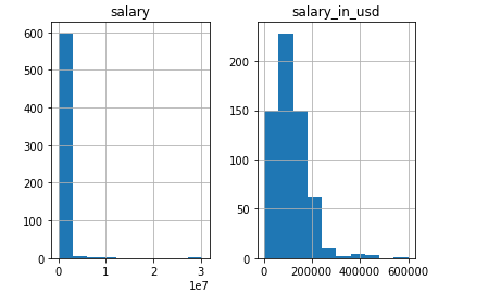
# lets fix the distribution of these to be normal
from scipy import stats

lambdas = []

for i,col in enumerate(numerical):
    if i == 0:
        R = X.copy()
    else:
        R = R.copy()

    R[col+'_box_cox'], L  = stats.boxcox((np.log(R[col])))
    lambdas.append((L,col,'+log'))

# improvements
R[['salary_box_cox','salary_in_usd_box_cox']].hist()
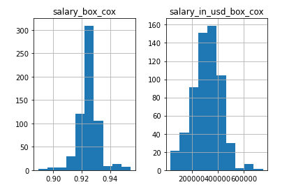
# almost there, just finalize the dataset
cata = pd.get_dummies(X,columns=categorical, drop_first=False)

cata['salary_in_usd_box_cox'] = R['salary_in_usd_box_cox']

cata.drop(columns=['salary','salary_in_usd'])

##### ******************* #############

# finally, let's test our stratify
# note, there is possible dataleakage from taking boxcoxs before splitting!!
# but to not make this very long, we will continue

from xgboost import XGBClassifier
from sklearn.metrics import confusion_matrix,classification_report
from sklearn.metrics import roc_auc_score, roc_curve, matthews_corrcoef


#stratify test
accuracy_stratify = []

random_splits = [i for i in range(1,25,2)]

for each_random_split in random_splits:

    X_train, X_test, y_train, y_test = train_test_split(cata, y,\
                                                    test_size=0.10,\
                                                    random_state=each_random_split,\
                                                    stratify=y)

    print(f'Trainning Set: {len(X_train)}')

    clf = XGBClassifier()

    clf.fit(X_train, y_train)

    y_pred = clf.predict(X_test)

    print(classification_report(y_test, y_pred),'\n')
    print(confusion_matrix(y_test, y_pred),'\n')

    print(matthews_corrcoef(y_test, y_pred))

    accuracy_stratify.append(matthews_corrcoef(y_test, y_pred))


#non-stratify test
accuracy_non_stratify = []

for each_random_split in random_splits:

    X_train, X_test, y_train, y_test = train_test_split(cata, y,\
                                                    test_size=0.10,\
                                                    random_state=each_random_split)

    print(f'Trainning Set: {len(X_train)}')

    clf = XGBClassifier()

    clf.fit(X_train, y_train)

    y_pred = clf.predict(X_test)

    print(classification_report(y_test, y_pred),'\n')
    print(confusion_matrix(y_test, y_pred),'\n')

    print(matthews_corrcoef(y_test, y_pred))

    accuracy_non_stratify.append(matthews_corrcoef(y_test, y_pred))

# remember, we did a bunch of tests
# we will want the average from each
print(f'\n\nStratify {(sum(accuracy_stratify)/len(accuracy_stratify))} vs \
            Non-Stratify {sum(accuracy_non_stratify)/len(accuracy_non_stratify)}')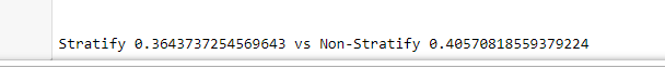
We see that in this example, the average Matthews Correlation Coefficient (A multi-class “accuracy” score for classification) is higher for our non-stratify class.
In this example, we benefitted from random sampling.
If you’re still confused about if you should use stratified sampling or not, implement cross-validation and see if your scores improve.
If they do, the sampling technique has helped you; if not, don’t implement it and stick with random sampling.
More information can be found on the usage of get_dummies() here.